If you have to work with files with evident geometrical distortions caused by microscope scanner you can correct calibration during processing. In order to do this you must have an additional image of calibration lattice or features on the image which can be used for calibration, i.e. features of known size. Calibration file can be created by the following steps:

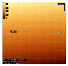
• Mark polyline nodes with known distance between them on the image of calibration sample using Curve Selection tool.

• Use the menu command Operations → Create Calibration Curve, window with two columns will pop up (calibration table). The left column contains parameters (numbers and measured segments’ lengths), the right column contains values to be set. Edit the right column, enter the known lengths between nodes (period of calibration lattice, for example).

• If you want to cancel the changes click the Cancel button. To save the file, click the OK button. On the suggestion of the program save the file to a desired place on hard drive.
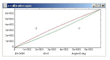
• After that the program will plot two calibration curves (x-calibration and y-calibration-slow) for x and y axes. The X (or Y) projections of polyline points marked on the image are plotted on horizontal axis, the true values of the same points are plotted on vertical axis. Then the program plots a graph marked by the green line, the red curve is a result of a reflection in a bisecting line of an angle formed by the coordinate axes. This curve is used for correction of a voltage controlling piezoelectric manipulator.

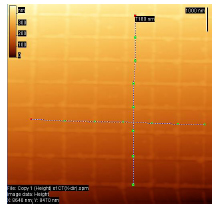
There is one remark: if Y (or X) projections are too small which can happen when the polyline is almost parallel to one projection axis (high accuracy is reached) and perpendicular to the other axis (large error arises). In this case one curve must be plotted for fast and slow scanning directions: x-calibration and y-calibration-slow. In order to do this plot two polylines on the image so that there are ‘good’ projections on both axes. To plot the second polyline independently from the first one mark the first node of the second line holding down the Ctrl key. It is possible to enter the same file name for both curves, the data will be saved in different sections according to orientation of the curve (along X or along Y).

The program automatically saves data for preferred direction. This direction is identified by a ratio of projections. If the polyline projection on one direction is 3 times larger than projection on the other direction then the first direction is considered a preferred direction and data for the second direction is not saved.

Calibration coefficients for slow and fast scanning directions along the same axis are substantially different. That is why the resulting calibration file can only be used for correction of images obtained with the same scanning direction (in the case described above X is scanning direction and rotational displacement of the scanner is 0°). To obtain hysteresis calibration for both scanning directions it is necessary to do the same operations with an image of test sample scanned along Y direction. The data can be saved in file with different name and then both files can be combined into one, but also you can save the data in the same file. It will be saved in x-calibration-slow and y-calibration sections. In order to work with images obtained with arbitrary scanning direction the calibration file must be created separately.

To apply obtained calibration data use function Mathematics → Dewarping.