Crystal surfaces can have steps. It is caused by crystal layer-by-layer growth. Each new layer forms a step on the previous one. As the layer grows the step grows as well gradually moving. The menu command Operations → Find Steps can be used in description of step growth with time. To use this function you need to take an image obtained by microscope working in special mode in which the same line is scanned through time.

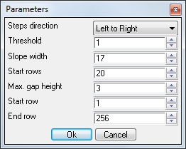
The Find steps command calls up a dialog window

.

In the window you choose the direction of analysis: from left to right if the top step is on the left and the bottom one is on the right, or from the right to the left in the opposite case.

The steps are identified by sudden changes in derivative. To calculate the derivative a convolution with kernel (1,0,-1) or (-1,0,1)is carried out, i.e. row of values is multiplied by vector (1,0,-1) for left-to-right direction or by (-1,0,1) vector for right-to-left direction. The operation is carried out from bottom to top beginning with the row specified in the Start row field and to the row specified in the End row field. Then a root-mean-squared deviation is calculated for the obtained derivative – RMS (feature height dispersion) and its filtered with threshold x specified in the field Threshold according to formula , Everything below the threshold is discarded and local maxima are found among points above the threshold. 1 is assigned to a point if there is the local maximum and 0 is assigned to it if there is no local maximum. Window width for detecting local maxima is specified in Slope width field. This operation is carried out with a few first rows the number of which is specified in Start rows field. The results are summed.

The local maxima are then looked for in the obtained row. Maximum in initial data is defined in the vicinity of the local maxima and obtained point is considered to be the beginning of a step. For each next row the maximum is searched only in the vicinity of maximum in previous row. If there is no maximum then the row is skipped. The amount of skipped rows can not exceed the number specified in the Max. gap height otherwise the step stops. If there is a maximum within the maximum gap then it is connected with previous maximum by a straight line.

When all the parameters are set click the OK button.

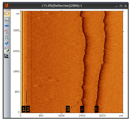
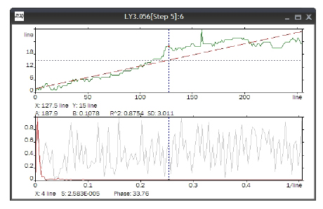
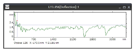
The steps are highlighted on the image and the step coordinate X is plotted as a function of time Y for each step. When vertical line is moved on one of the graphs a new window displaying horizontal section of the surface along the step pops up. The command Curve → Fitting can be used to level the current horizontal section (remove average slope).

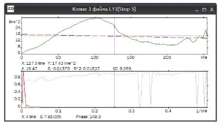
The coordinate function can be auto-correlated by command Curve → Auto-correlation. And the command Curve → Structure function provides a structure function according to formula:

It is easy to see that correlation function and structure function are symmetrical.

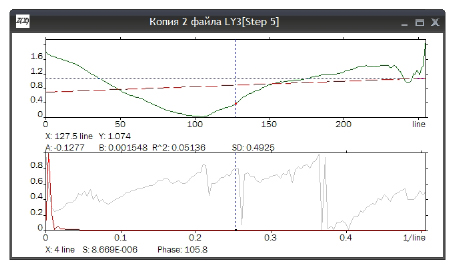
Horizontal section of the surface along the step №5:

.

Correlation function:

.

Structure function:

.